
Laboratory 8
System of Linear Equations
This laboratory activity aims to implement the principles and techniques of solving linear equations using the various linear algebra techniques and to solve a system of equations using Python programming.
The practices of the activity include working around with the system of linear equations using Python programming. This activity implies and teaches the various algebra techniques in solving linear equations. Moreover, the deliverables of the activity are to provide an equation and solve it using the NumPy functions. Lastly, it was achieved by creating a scenario and represent it in a matrix then solve using Python programming and NumPy function.
The results from solving a system of linear equations from the scenario created using the linear equation and the np.linalg.solve() function from NumPy are presented in this section.
Scenario
I and my brother have a collection of anime figurines and I created a list for our current figurines and the one that is still currently in a pre-ordered state. In total, we currently have 6 nendoroids, 4 Figma, and 3 pop up parade. This cost us a total of 30,000. Meanwhile, the current figurines we pre-ordered that will be released in the future are 2 nendoroids, 2 figma, and 3 pop up parade, for a total of 18,000. I am still waiting for the other re-release of the figures I failed to acquire. Those are 4 nendoroids, 2 Figma, and 1 pop up parade which will be about 15,000.
System of linear equation
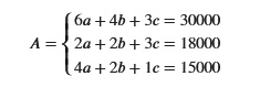
The Figure above is the system of linear equation form of the values or elements from the given scenario
Coding
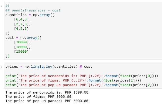
Code snippet above shows the code created for solving a linear equation using the inverse equation or the inverse function with a dot product from the NumPy library. The results show the prices of each figurine from the given equations.
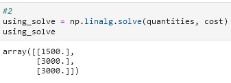
Figure above shows the results from solving a system of the linear equation using the np.linalg.solve() function from NumPy. In comparison with the result from solving it with an inverse equation or inverse function with a dot product, it can be observed that both of the results are identical. The function np.linalg.solve() according to [1], “computes the “exact” solution, x, of the well-determined, full rank, linear equation ax = b” This is the reason why the answers are the same.
So what’s this all about?
This laboratory familiarized you with the principles and techniques of solving linear equations using the various linear algebra techniques and to solve a system of equations using Python programming and NumPy library. You learned how this can be implemented through the practical examples provided in the discussion.
Real-world application
The essence of the system of linear equations is that it can represent data or elements in life which can help us to make our life easier. This is evident in the practical examples presented in this laboratory and solving linear equations help in producing technologies like the one that is used today in the medical field which is CT imaging [2]. According to [3], linear algebra is fundamental in robotics because it was used for robot modeling, control, and optimization. An equation or a mathematical model represents how the arm of a robot moves and every joint of this can be described using a matrix and a proper matrix operation here can result in another equation that might describe a specific position of the arm of the robot [4]. To conclude, a system of linear equations can be used to model the kinematics of a robot arm.
References
[1]”numpy.linalg.solve — NumPy v1.19 Manual”, Numpy.org, 2020. [Online]. Available: https://numpy.org/doc/stable/reference/generated/numpy.linalg.solve.html. [Accessed: 13- Dec- 2020].
[2]L. Flores, V. Vidal, and G. Verdú, “System Matrix Analysis for Computed Tomography Imaging”, plos.org, 2015. [Online]. Available: https://journals.plos.org/plosone/article?id=10.1371/journal.pone.0143202. [Accessed: 12- Dec- 2020].
[3]N. Ratliff, “Linear Algebra and Robot Modeling”, Ipvs.informatik.uni-stuttgart.de, 2020. [Online]. Available: https://ipvs.informatik.uni-stuttgart.de/mlr/wp-content/uploads/2014/04/advanced_robotics_ss14_lecture1_notes1.pdf. [Accessed: 13- Dec- 2020].
[4]M. Steglehner and B. techn, “Flexible solutions of polynomial systems and their applications in robotics”, Maplesoft.com, 2020. [Online]. Available: https://www.maplesoft.com/Whitepapers/MichaelSteglehner.pdf. [Accessed: 13- Dec- 2020].