
Laboratory 6
Matrices
This laboratory activity aims to implement the principles and techniques of performing basic matrix operations, translating matrix equations and operations using Python, and to be familiar with matrices and their relation to linear equations.
The practices of the activity include translating matrix equations and performing different basic matrix operations using Python. This teaches and implies the techniques of doing operations between matrices with the use of Python and NumPy library. The deliverables of the activity are to provide a code or a function that will display all the details of a matrix that has been discussed in this laboratory and to perform operations between matrices. It was achieved by using some functions from the NumPy library such as np.shape() that returns the shape of an array [1], np.ndim() that returns the number of array dimensions [2], np.all() that test whether all array elements along a given axis evaluate to True [3], np.identity() for producing an identity array [4], np.zeros() which “return a new array of given shape and type, filled with zeros” [5], np.ones() that returns an array filled with ones [6], np.array_equal() that returns True if the two arrays have the same shape and elements and False otherwise [7], np.sum() that sum up the elements of the array over a given axis [8], np.multiply() that “Multiply arguments element-wise” [9].
Activity 1 Flowchart
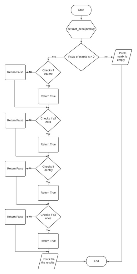
Figure above shows the flow of the function created that thoroughly describes a matrix about its shape, size, rank, whether it is a square or a non-square, an empty matrix or not, an identity matrix, zeros, or ones.
Activity 2 Flowchart
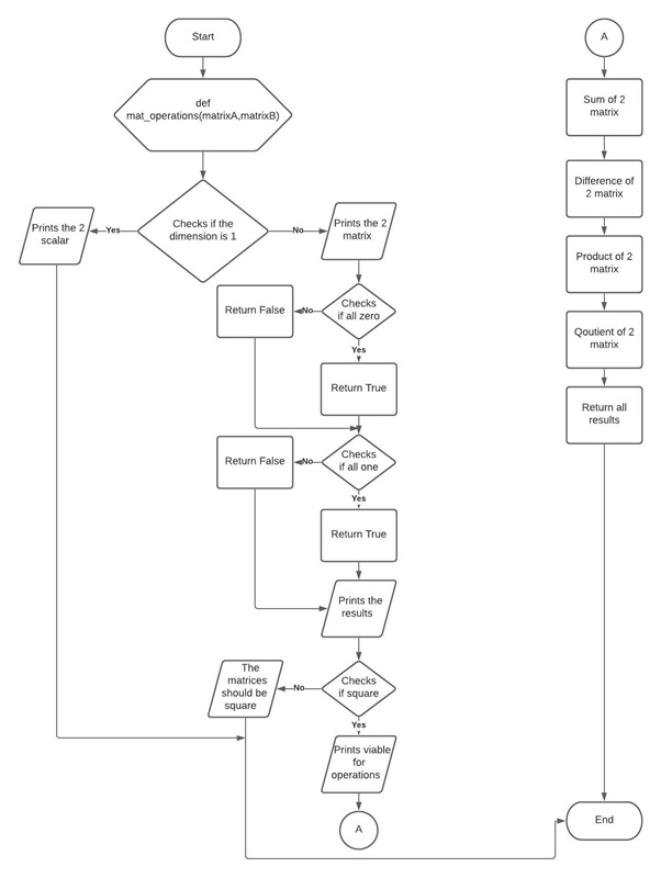
Figure above shows the flow of the function created that takes two matrices or scalars and displays the description of a matrix if it is a matrix otherwise it prints the scalars. The function also determines if the matrices are viable for operation, and if it is, it will return the sum, difference, element-wise product, and element-wise division of matrices.
The result of the two activities done by implementing the principles and techniques observed in the discussion in this laboratory which all about performing basic matrix operations and translating matrix equations was presented in this section.
Activity 1
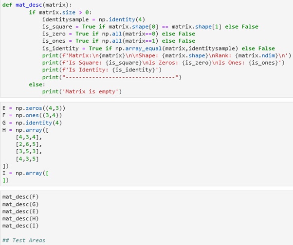
Figure above shows the code of block created to come up with a function that describes the matrix. Starts by creating a function named “mat_desc” that takes one parameter. Next, the size of the matrix was identified to determine if the matrix is an empty matrix or not. The creation of an identity matrix was done to have a basis if the matrix passed into the parameter of the function is identical to it and if it is, hence it can be said that the matrix passed into a parameter is an identity matrix. Moreover, to identify if the matrix is a square, its rows and columns were tested if equal to each other using the np.shape() function. The matrix was identified if it is a matrix of one or a matrix of zero by checking the elements of it first if it is all one and then if it is all zero. Lastly, the results were printed to present the description of the matrix based on the codes created.
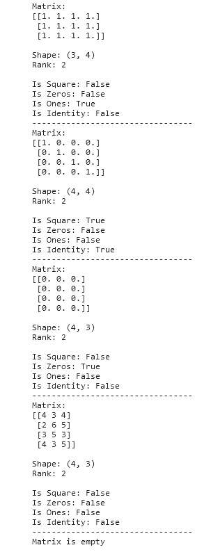
The output using the function created to describe a matrix. Each sample presented is specifically created to test out each line of code that determines what kind of matrix it is. It can be observed that the function is working well since it returns False when the matrix doesn’t satisfy the condition on each line of code and it returns True when it satisfied the condition.
Activity 2
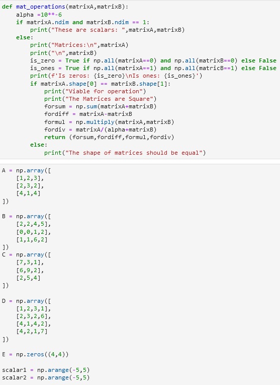
Code snippet above shows the code of block created for a function that demonstrates the basic operations on matrices using Python. First, to identify if the passed values on the 2 parameters of the function are scalars or a matrix, the dimension of it was tested out. If the dimension is 1 then it is a scalar that is created using np.arange() function else it as a matrix. The program will end if it found out that it is a scalar while if it is a matrix, it will then display the description of a matrix and it will test out if the 2 matrix has the same shape. If the shape of the 2 matrices is different from one another, the program will display an error message and end the program while if it has the same shape, it will display that the matrices are viable for operation and proceed on performing the block of code created to demonstrate the different operations can be done between the matrices. This includes the sum, difference, element-wise product, and element-wise division of matrices.
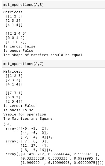
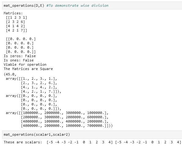
The Figures above shows the output of different matrices used in using the function created for performing different operations. The output for the 4 operations done is as follows: sum, difference, element-wise product, and element-wise division of matrices. The focus of the program is to follow the instruction given which states to return the values. The other way to present the results from the operations is to print the resulting values after a short definition that the value is a result of that line of code.
So what’s this all about?
This laboratory introduced the concept of matrices and demonstrate some basic operations that can be done between the matrices. It was discussed that matrices are representations of complex equations or multiple inter-related equations from 2-dimensional equations to even thousands of them. What you have achieved in this laboratory is the learnings about the basic rules when performing operations between matrices like the shape of the matrices should be the same.
Real-world application
The application of matrix computation can be observed in creating large-scale models since according to [10], “In others, like direction learning and topic modeling, the matrix parameter instead pops up in the algorithms as the natural tool to represent uncertainty.” In addition, the emergence of large matrices in different applications brought new algorithms and tools [10]. You have learned and realized how important the concept of matrices in different fields because of this laboratory. The operations you have seen in this laboratory are important to understand deeper the next concepts or application of the matrices. According to [10], matrices can be used to find the interrelations between features or for example, how feature (A) related to feature (B).
Matrix operations play an important role in solving a problem in agriculture. There was a book published that presents the PAM approach or Policy Analysis Matrix approach way back in 1981. This approach was developed by the researchers at the University of Arizona and Stanford University to study the changes in agricultural policies in Portugal [11]. Since then, PAM has become well known for providing information to help the policymakers address three central issues of agricultural policy analysis such as the competitiveness of agricultural system, impact of new public investment in infrastructure, and agricultural research or technology on the efficiency of the systems [11]. A matrix in this case follows two rules of accounting, the first is defining the relationship across the columns of the matrix and the second is defining the relationship down the rows of the matrix [11]. The data in the matrix are all about the revenues and costs etc. and performing specific operations on this data results in a new variable that represents another data about a specific scenario for example. Overall, doing calculations using operations on these variables might result in good or bad values which will be interpreted to find out it will make better the agricultural system.
References
[1]”numpy.shape — NumPy v1.20.dev0 Manual”, Numpy.org, 2020. [Online]. Available: https://numpy.org/devdocs/reference/generated/numpy.shape.html. [Accessed: 31- Oct- 2020].
[2]”numpy.ndarray.ndim — NumPy v1.19 Manual”, Numpy.org, 2020. [Online]. Available: https://numpy.org/doc/stable/reference/generated/numpy.ndarray.ndim.html. [Accessed: 31- Oct- 2020].
[3]”numpy.all — NumPy v1.19 Manual”, Numpy.org, 2020. [Online]. Available: https://numpy.org/doc/stable/reference/generated/numpy.all.html. [Accessed: 31- Oct- 2020].
[4]”numpy.identity — NumPy v1.19 Manual”, Numpy.org, 2020. [Online]. Available: https://numpy.org/doc/stable/reference/generated/numpy.identity.html. [Accessed: 31- Oct- 2020].
[5]”numpy.zeros — NumPy v1.19 Manual”, Numpy.org, 2020. [Online]. Available: https://numpy.org/doc/stable/reference/generated/numpy.zeros.html. [Accessed: 31- Oct- 2020].
[6]”numpy.ones — NumPy v1.19 Manual”, Numpy.org, 2020. [Online]. Available: https://numpy.org/doc/stable/reference/generated/numpy.ones.html. [Accessed: 31- Oct- 2020].
[7]”numpy.array_equal — NumPy v1.19 Manual”, Numpy.org, 2020. [Online]. Available: https://numpy.org/doc/stable/reference/generated/numpy.array_equal.html. [Accessed: 01- Nov- 2020].
[8]”numpy.sum — NumPy v1.19 Manual”, Numpy.org, 2020. [Online]. Available: https://numpy.org/doc/stable/reference/generated/numpy.sum.html. [Accessed: 01- Nov- 2020].
[9]”numpy.multiply — NumPy v1.19 Manual”, Numpy.org, 2020. [Online]. Available: https://numpy.org/doc/stable/reference/generated/numpy.multiply.html. [Accessed: 01- Nov- 2020].
[10]”Large Scale Matrix Analysis and Inference”, Stanford.edu, 2020. [Online]. Available: https://stanford.edu/~rezab/nips2013workshop/. [Accessed: 01- Nov- 2020].
[11]Repository.ruforum.org, 2020. [Online]. Available: https://repository.ruforum.org/system/tdf/Introduction%20to%20the%20%20Policy%20analysis%20Matrix%20by%20Scott%20Pearson.pdf?file=1&type=node&id=33614&force=. [Accessed: 01- Nov- 2020].