
Laboratory 4
Vector Operations
This laboratory activity aims to implement the principles and techniques of doing the operations between the vectors using Python and to visualize the vector operations.
The practices of the activity include being familiar with different operations that can be done between the array of vectors and to make functions that will solve operations following a certain formula. This also teaches and implies the techniques of doing operation between an array of vectors and visualizing the resulting vector using a 3D-plot. The deliverables of the activity are to provide a function that will solve the modulus of a vector using the Euclidean Norm formula, a function that will solve the inner product of two vectors using the inner product formula, and to code the operation of vectors given by the instructor also, explain its resulting vector using a 3D-plot. Lastly, It was achieved by implementing loops on the function created and provide specific operations to solve the modulus of vector and inner product of two vectors. The expected value in the last task was achieved by implementing the operation vectors introduced in this laboratory and it was visualize using a 3D-plot.
Activity 1 Flowchart
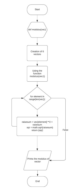
Figure above shows the flowchart of the function created that solves the modulus of a vector. A function named ‘modulus’ was defined first and it has a parameter ‘vec’ so that it can receive the value of the vector. When the values of vectors are created and were passed into the ‘vec’ of the ‘modulus’ function, the loop will be taking that values and it will perform the operations created inside the loop and the number of times it will execute the loop is based on the number of items in a created list of values or length of the vector. Afterward, the computed values will be returned and printed.
Activity 2 Flowchart
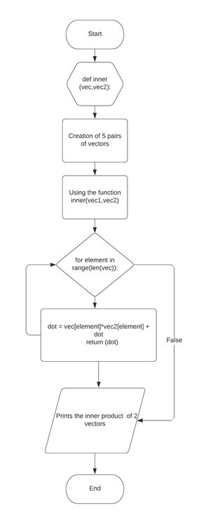
The flowchart of the code for the function created that solves the inner product of the vectors using the inner product formula. The function was defined first and when the values of the pair of vectors were passed to the parameter of this function, these values will be used in the loop created that contains the operations to solve the inner product of the 2 vectors. The loop will continue looping until the elements of vectors were used and the result can be printed after the result from the loop was returned.
Activity 3 Flowchart
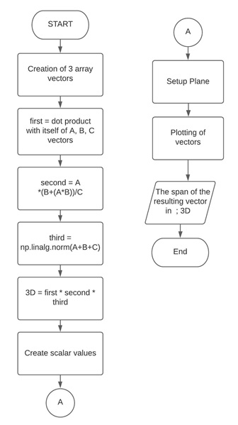
Figure above shows the algorithm created to get the resulting vector of the 3 vectors by doing the operations on the given vectors. The creation of 3 array vectors given by the instructor was done first. The operations are sliced into 3 steps to easily visualize or to make the debugging on the program easier if the result doesn’t match the expected value of the resulting vector. Followed by arranging values to be used as scalar values and setting up the 3-dimensional plane. Lastly, it was plotted and shown at the same time with the resulting vector.
The result of the activities done by implementing the techniques and principles of doing the different operations between vectors to solve specific problems like getting the modulus of vectors or the inner product of two vectors are presented in this section.
Activity 1
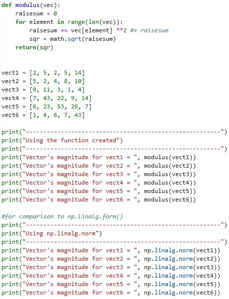
Figure above shows the code of block created to have a function that calculates the modulus without using the function from the NumPy library. The variable “raisesum” was set to 0 so that the assignment of this variable is possible at the same time that it was used as referenced. A loop statement was created to access every element inside the vectors created and inside this loop statement are the operations that will compute the modulus of the 6 different vectors. The operations include the summation of the squared elements from the vectors. The sum of these elements was assigned to the “raisesum” variable and the square root of this was assigned to “sqr” which was returned afterward and printed. The second part of the code is for the comparison between the function created and the function from the NumPy library.
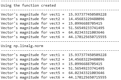
The output from using the modulus function created and the output from using the np.linalg.norm() function from NumPy library. It can be observed that using the basic operations in the modulus function created produced the same result with the np.linalg.norm()function.
Activity 2
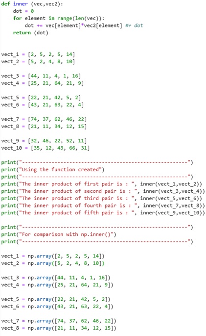
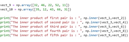
The Figure above shows the code of block created to show the difference between the results from using the function from the NumPy and the function created that involves vector operations. The inner() function created contains a loop that will run based on the number of elements inside the list created to represent a vector. It gets the values from the parameters of inner() function which is the ‘vec’ and ‘vec2’ that holds the values being passed when the list of vectors used as an argument when calling the function or in code, ‘inner(vect_1,vect_2)’. The operations inside the loop now have an access to the elements hence it can do the operations properly and return the result.
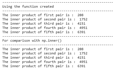
The output from using the function created and using the np.inner() function from the NumPy library. It can be observed that the resulting values from using the function created are identical with the resulting values from using the np.inner() function.
Activity 3
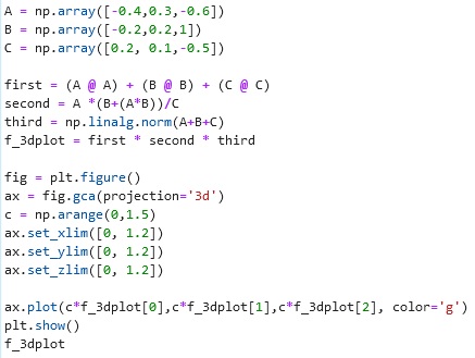
The block of code created to solve the vector operation using the given vector values. After analyzing the problem, the first part of the operation was coded first, and it can be observed that the square of the vector was done by getting the dot product of itself because according to [1], “The projection of a vector on to itself leaves its magnitude unchanged, the dot product of any vector with itself is the square of that vector’s magnitude.” It was followed by calculating the second and third parts then the multiplication of each part to get the resulting vector. To visualize the resulting vector, the values were plotted into a 3-dimensional plane using the plot instead of the quiver to see how the continuous line of this behaves or to show all the possible vectors it can reach using the scalar values.
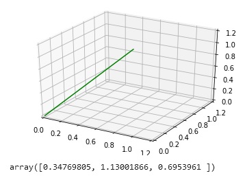
The resulting vector and the visualization of it using a 3D plot. The line represents the transformed values from the resulting vector by scaling the values with the arbitrary constant or by multiplying each of these into the scalar values created to show the span of it. The values achieved are the same as the expected values by the instructor.
So what’s this all about?
This laboratory demonstrated the concepts behind the different principles and techniques that can be implemented when working on the operation between vectors. You got to familiarize yourself with the different operations that can be used or the other forms of the specific operation. For example, when dividing, the function np.divide() can be used or simply the slash ‘/’. Moreover, the other operations too can be done just by using the Python built-in function but using the NumPy library functions can make our life easier for solving specific problems that require multiple operations such as getting the magnitude of a vector. It was shown in this laboratory through discussion and the activities how long the code will be if we try to make a function to solve using the formula compare by using the functions from NumPy library specifically the np.linalg.norm() for computing the magnitude of a vector and the np.inner() for computing the inner or dot product of two vectors. You also learned through the activity given that the dot product of any vector with itself is the square of that vector’s magnitude [1].
References
[1]”Vector Multiplication – The Physics Hypertextbook”, The Physics Hypertextbook, 2020. [Online]. Available: https://physics.info/vector-multiplication/. [Accessed: 24- Oct- 2020].