
Laboratory 3
Linear Combination and Spans
This laboratory activity aims to implement the principles and techniques of representing linear combinations in the 2-dimensional plane. This also aims to visualize spans using vector fields in Python and to perform vector field operations using scientific programming.
The practices of the activity include combining linear scaling and the addition of a vector. This activity teaches and implies the techniques of representing linear combinations in the 2-dimensional plane and visualizing spans using vector fields in python. Some functions were used such as np.arange() function that returns evenly spaced values within a given interval [1], plt.scatter() function that makes the plotting of the x and y components of a vector into a plane faster [2], plt.axhline() and plt.axvline() functions that adds a horizontal and vertical line across the axes [3][4], np.meshgrid() function that returns coordinate matrices from coordinate vectors [5]. The deliverables of the activity are to provide a linear equation and vector form of the linear combination. It was achieved by providing random values to be used in the equations and the vector form of the linear combination.
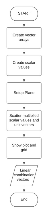
Activity 1 Flowchart
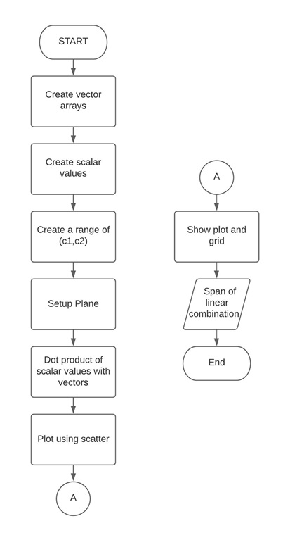
Activity 2 Flowchart
The result of the two activities done by implementing the principles and techniques of representing combinations in the 2-dimensional plane and visualizing spans using vector fields by performing operations using scientific programming was presented in this section.
Activity 1
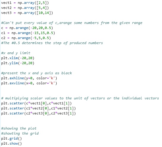
The code snippet above shows the code of block created to show the linear combination visualization. It was achieved by first creating 3 different arrays of vectors and arranging 3 different scalar values by using the np.array() function and np.arrange() function. The step used in 3 different scalars is 0.5. The linear combinations are created by multiplying the scalar values to the unit vectors or the individual vectors. Lastly, these linear combinations in 1 vector were plotted into a 2-dimensional plane using the plt.scatter() function.
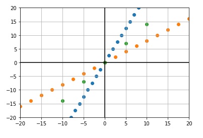
The Figure above shows the output of 3 linear combinations in 1 vector. Each combination intersects in the origin and makes a line and it can be observed that they are not linearly dependent on each other.
Activity 2
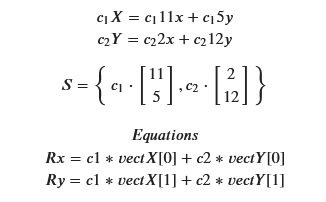
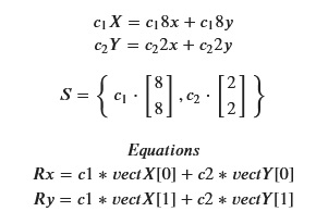
The 2 vectors and the equations to be used in getting the span visualization of the first linear combination of two vectors.
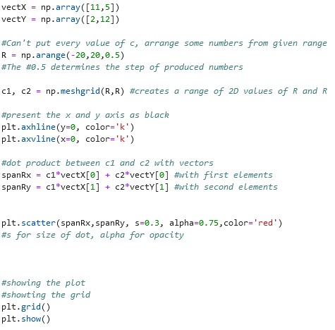
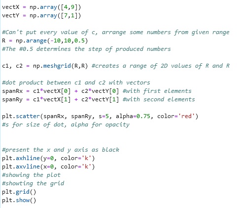
The block of code above is created to present the span of the first linear combination of two vectors. Two arrays of the vectors were created and the creation of scalar values was done using the np.arrange() function and this time with the np.meshgrid() function to create a range of 2D values of R and R. A dot product was performed between c1 and c2 with the array of vectors are done using the equations to get the spanRx and spanRy. Lastly, this was plotted into the plane using the plt.scatter().
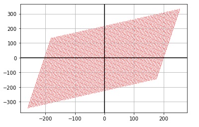
The figure above shows the output of the code executed to present the span of the first linear combination of two vectors. All the specific vectors inside the plane that was created using the equation are shown. The vectors are not a scale of each other therefore it is not linearly dependent and it has a rank of 2.
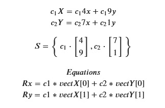
The 2 vectors created and the equations to be used in getting the span visualization of the second linear combination of two vectors.
The block of code created to show span visualization of the second linear combination of two vectors that will be produced from the array of vectors and scale values. The code and functions used and how the plane and plot showed were the same as the first code presented in this activity. The only changes made are the values of the array of vectors.
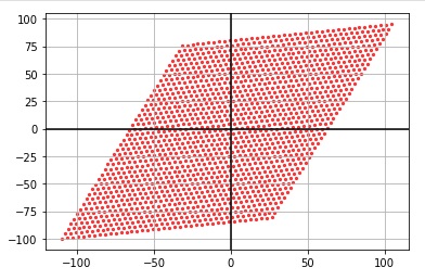
Figure above shows output or the span of the second linear combination of two vectors. It can be observed that all the set of vectors were plotted and it was linearly independent since the vectors are not a scale of each other nor they aligned. It also has a rank of 2.
The 2 vectors used and the equation for getting the span visualization of the third linear combination of two vectors.
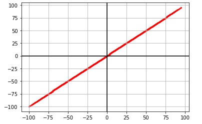
The output of the plotted values from the third linear combination of two vectors. It can be observed that the span is a colinear vector or aligned hence it is a linearly dependent vector and has a rank of 1.
Note:
The role of unit vectors is to have a value if the purpose is to reach a specific span since when the scalar was multiplied to these unit vector, it transforms that unit vector or stretches it out into a plane [6]. Also, the scalar values multiplied to the unit vectors tell where the given vectors will land in graphical representation or plane.
So what’s this all about?
The implementation of the principles and techniques of representing linear combinations in the 2-dimensional plane are learned through the discussion in this laboratory and the given activities by the instructor. Using the vector fields in Python and by performing vector field operations using scientific programmings such as doing a dot product between the scalar values and vectors, the spans were visualized. You have learned new functions in this laboratory such as the plt.scatter() function that makes the plotting of the x and y components of a vector into a plane faster [2]. The np.arange() functions that create numbers from the given interval [1]. You also learned that the span can be linearly dependent vector when it is a scale of one another otherwise it is an independent vector. Moreover, for every linear combination, there would be a distinct set of values or plotting unless it is a linearly dependent vector. If a span is linearly dependent, it has a rank of 1 and if the span is presented in a 2-dimensional plane then it has a rank of 2. To conclude, the span of the two vectors represents all the possible vectors you can reach using only the two vector field operations which is vector addition and scalar multiplication. Also, the scalar values scale the unit vectors or tell where the vector will land in the plane.
Real-world application
The concept of linear combination can be applied in engineering especially computer engineering or in some programming-related courses in a way that some programs need to do the concept of linear combination because of the specific purpose of the program. For example, a program that represents data through vectors that are plotted in a plane. This program can be about showing all the specific position of something like how is the movement of an eagle at a specific time. We can plot it using a linear combination and in this way, we can see the span of all possible location movements of the eagle during the specific time set.
References
[1]”numpy.arange — NumPy v1.19 Manual”, Numpy.org, 2020. [Online]. Available: https://numpy.org/doc/stable/reference/generated/numpy.arange.html. [Accessed: 22- Oct- 2020].
[2]”matplotlib.pyplot.scatter — Matplotlib 3.3.2 documentation”, Matplotlib.org, 2020. [Online]. Available: https://matplotlib.org/3.3.2/api/_as_gen/matplotlib.pyplot.scatter.html. [Accessed: 22- Oct- 2020].
[3]”matplotlib.pyplot.axvline — Matplotlib 3.3.2 documentation”, Matplotlib.org, 2020. [Online]. Available: https://matplotlib.org/3.3.2/api/_as_gen/matplotlib.pyplot.axvline.html. [Accessed: 22- Oct- 2020].
[4]”matplotlib.pyplot.axhline — Matplotlib 3.3.2 documentation”, Matplotlib.org, 2020. [Online]. Available: https://matplotlib.org/3.3.2/api/_as_gen/matplotlib.pyplot.axhline.html. [Accessed: 22- Oct- 2020].
[5]”numpy.meshgrid — NumPy v1.19 Manual”, Numpy.org, 2020. [Online]. Available: https://numpy.org/doc/stable/reference/generated/numpy.meshgrid.html. [Accessed: 22- Oct- 2020].