
Laboratory 2
Plotting Vector using NumPy and MatPlotLib
This laboratory activity aims to implement the principles and techniques of plotting a vector with the use of the MathPlot library for creating visualizations in Python and the NumPy library for fast operations on arrays.
The practices of the activity include creating arrays and plotting of vectors. This teaches and implies the techniques of manipulating arrays and plotting of vectors. The deliverables of the activity are to provide an array and formulas needed to completely plot the vectors. Lastly, it was achieved by reading the documentation of the functions.
The results from the activities done by implementing the principles and techniques of representing the vectors through plotting using the MathPlot library and NumPy library to manipulate arrays were presented in this section. The first activity was focused on providing necessary formulas to complete the code while the second activity was all about code analysis and how to transform a project that lacks coding conventions into a well-created project that follows coding convention. Lastly, the third activity was about understanding the relationship of each vector used to represent data.
Activity 1
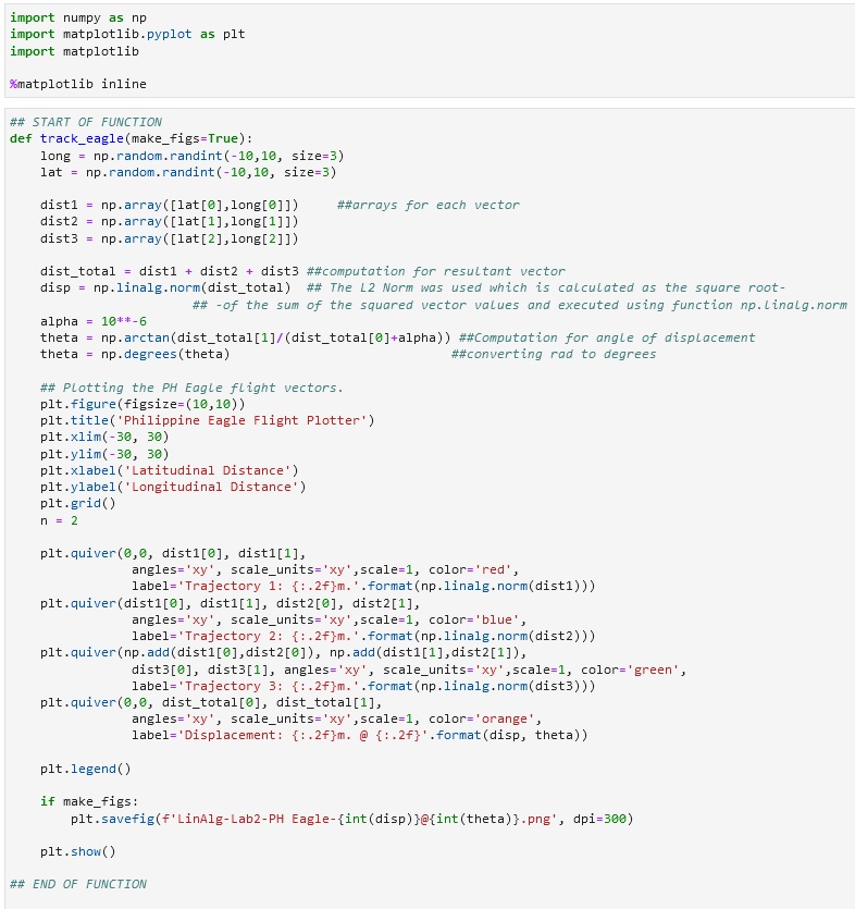
The code snippets above show the code executed and the sample output or the Philippine Eagle Flight Plotter. The task was to fill in the necessary codes to make the function works. Three 2-D arrays were created which are assigned into dist1, dist2, and dist3 variable from the long and lat variable which generates random integers. In computing the total distance, the computation of three arrays was performed in the dist_total variable therefore, it holds the value of the summation of dist1, dist2, and dist3. The magnitude of the displacement was computed next which is assigned into disp variable and the L2 norm was used which is calculated as the square root of the sum of the squared vector values and executed using the function np.linalg.norm. The angle of the displacement was calculated next using the equation in Figure 1 which is np.arctan(dist_total[1]/(dist_total[0]+alpha)) wherein alpha has a value of 10^-6 so that the division over 0 never happened which will cause an error. and it was assigned to theta variable wherein after getting the result, the value of theta was converted into degrees using the code provided np.degrees from the Numpy library.
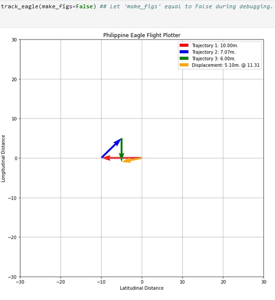
Proceeding to the plotting of vectors, plt.quiver was used because it plots a 2D field of arrows based on the parameter provided. As shown in Figure 1, the first vector was plotted using the line of code that includes plt.quiver (0,0, dist1[0], dist1[1]) this is the parameter used to identify the location of the arrow, the 0,0 is the origin of the tail of the arrow while the dist1[0] and the dist[1] is the head of the arrow. The code that follows this is for the modification of how the arrow will look and the code needed for the legend of the graph. The same concept was used in plotting the second vector and for the third, the addition of the first vector and the second is used as the origin of the tail and still used its value dist3[0] and dist3[1] for its arrowhead. The displacement was plotted using the values of variable dist_total and in the same line of code, for the legend, it includes the variable theta or the degree. The plt.legend() shows the legend at the right top side of the graph as shown in Figure 2 and the plt.show() show what is inside the plt or the vectors plotted in the canvas. Lastly, the track_eagle(make_figs=True) is the one that confirms if the saving of the graph into an image will be executed so, if it was set to False then no image will be saved.
Activity 2
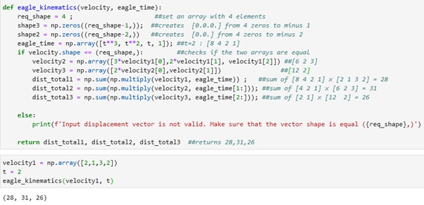
The code above shows the organized eagle_kinematics function that computes the distance traveled by the eagle. To begin, the req_shape = 4 set an array that has 4 elements or set the shape into 4 and it was followed by the creation of shape3 and shape2 variables that returns an array of zeros since np.zeros are used. The eagle_time or the first array with 4 elements was created by getting the value of ‘t’ which in this case was set to 2 by passing as an argument when calling the eagle_kinematics function and when it was substituted to the ‘t’ in the line of operation provided it results in [8 4 2 1]. The if statement in Figure 3 checks if the number of elements of the velocity variable is equal to the req_shape which has a shape of 4. Besides, the variable velocity1 passed its value to velocity since it is used as an argument in calling the eagle_kinematics function. Therefore, the velocity now has 4 elements too and equal to the shape or req_shape. The next line of code is for making the second array of velocity. The velocity2 variable created an array with 3 elements by multiplying to 3 the first element of variable velocity1 or the 2 which results in 6 and multiplying to 2 the second element of variable velocity1 or the 1 which results in 2 and lastly, getting the third element of the variable velocity1 or the number 3. Overall, the velocity2 now has [6 2 3]. Next, velocity3 created an array with 2 elements by multiplying to 2 the first element of velocity2 or the 6 and getting its second element which results in [12 2]. Now, the set of velocities are present, and the computation of distance is possible by manipulating the array of eagle_time to match the number of elements for each set of velocities. The values of eagle_time were sliced to match the number of elements or the shape of each array of velocities. The first total distance computed using the equation provided from the first arrays with 4 elements results in 28 while the second total distance from the arrays with 3 elements results in 31 and lastly for the third total distance from the arrays with 2 elements results in 26. The three values from the total distance were returned so when the function was called, it will give the three total distances.
Activity 3
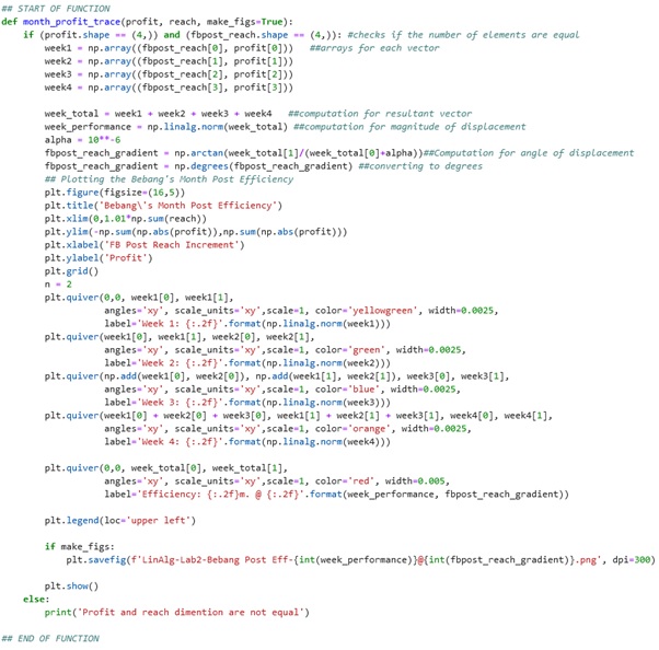
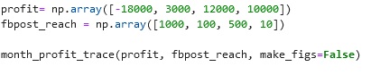
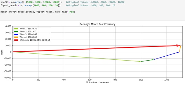
The code snippets above show the completed code for Bebang’s Project and the output or the result of Bebang’s month post efficiency. The values of the vectors come from the arrays of profit and fbpost_reach by making an ordered pair of the 2 arrays. The computation of the resultant vector, magnitude of the displacement, angle of displacement, and even in plotting the vectors are the same as what is used or concept implemented in plotting Philippine Eagle Flight Plotter.
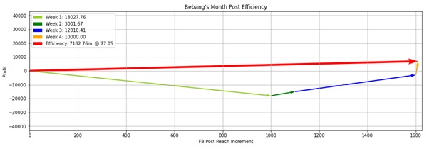
In the scenario above, the total value of profit was decreased. It can be observed in this scenario that the efficiency of Bebang’s post also decreased.
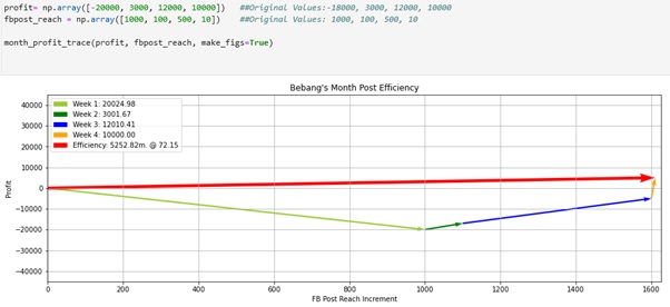
The total value of profit is increased and the efficiency of Bebang’s post also increased.
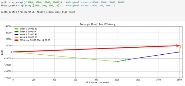
The fbpost_reach was manipulated into a lower value. The result proves that the lower fbpost_reach means lower efficiency of Bebang’s post.
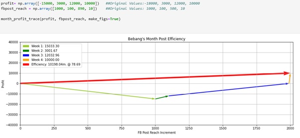
The result of the fourth scenario wherein the fbpost_reach was adjusted into higher value and this results in the higher efficiency of Bebang’s post.
To conclude, as shown in Figures 6 to 9, the higher the profit or the fbpost_reach of Bebang means, the higher the efficiency of its month post while the lower profit or fbpost_reach means lower efficiency of the month post. Therefore, the Bebang’s month post efficiency is directly proportional to profit and fb_post reach.
Used functions
The first function was used is the np.array which is used for creating an array [3]. The next is the one used in executing the L2 norm for computation of magnitude of displacement which is np.linalg.norm. It was defined according to its documentation [4], “This function can return one of eight different matrix norms.” It contains ord parameter which in this laboratory, the ord holds the L2 norm which is one of the eight different matrix norms and this is calculated as the square root of the sum of the squared vector values which is the formula in computing the magnitude of displacement [1]. The next function used is the np.arctan which is used in performing trigonometric inverse tangent [5] and the np.degrees which is used for converting angles from radians to degrees [6]. Moreover, in plotting the figures, plt.figure is used to create a new figure or activate an existing one [7]. The other function from the Mathplot library used in this laboratory includes plt.title – “Set a title for the axes.” [8], plt.xlim – “Get or set the x limits of the current axes.” [9], plt.ylim – “Get or set the y-limits of the current axes.” [10], plt.xlabel – “Set the label for the x-axis.” [11], plt.ylabel – “Set the label for the y-axis.” [12], plt.grid() – “Configure the grid lines.”, therefore if plt.grid is not used, there are no grid lines on the canvas [13]. Also, plt.quiver is used to plot a 2D field of arrows [2], plt.legend() is the one placing a legend on the axes [14], plt.show() is the one who display all open figures [15], plt.savefig is used to save the current figure [16]. Moreover, the np.zeros is used in the second problem in this laboratory and this function is used to return a new array of given shape and type which is filled with zeros [17]. The np.sum and the np.multipy are used to add the element on the array [18] or multiply the elements [19]. Lastly, the np.abs is used to calculate the absolute value of an element [20].
Real-world application
The vector is defined by mathematicians and scientists as a quantity that depends on the direction and when there is direction then also a force, acceleration, and displacement are involved [21]. These values in real-life are can be used to study one’s behavior just like the Philippine eagle flight plotter, by knowing the values researcher can come up with many conclusions. Vectors are also applied in playing basketball because the ball was being thrown into the air and this creates projectile and projectile can be represented with vectors.
Other examples of how vectors are used or other real-life situations that can be modeled using vectors are how the forces acting on a moving boat in the river. “The boat’s motor generates a force in one direction, and the current of the river of the river generates a force in another direction.” [22]. In this example, the direction of where the boat will go can be calculated when both the magnitude and direction of both forces from the current of the river and the force generated by the boat’s motor are known. Lastly, momentum vectors are applied in playing billiard since the players are trying to predict what will happen when the balls collide with the specific force exerted to the ball, the ball passes some of its momentum to the other ball when it collides because of the impact [23].
References
[1] J. Brownlee, “Gentle Introduction to Vector Norms in Machine Learning”, Machine Learning Mastery, 2020. [Online]. Available: https://machinelearningmastery.com/vector-norms-machine-learning/. [Accessed: 26- Sep- 2020].
[2]”matplotlib.pyplot.quiver — Matplotlib 3.3.2 documentation”, Matplotlib.org, 2020. [Online]. Available: https://matplotlib.org/api/_as_gen/matplotlib.pyplot.quiver.html. [Accessed: 26- Sep- 2020].
[3]”numpy.array — NumPy v1.19 Manual”, Numpy.org, 2020. [Online]. Available: https://numpy.org/doc/stable/reference/generated/numpy.array.html. [Accessed: 26- Sep- 2020].
[4]”numpy.linalg.norm — NumPy v1.19 Manual”, Numpy.org, 2020. [Online]. Available: https://numpy.org/doc/stable/reference/generated/numpy.linalg.norm.html#numpy.linalg.norm. [Accessed: 26- Sep- 2020].
[5]”numpy.arctan — NumPy v1.15 Manual”, Docs.scipy.org, 2020. [Online]. Available: https://docs.scipy.org/doc/numpy-1.15.1/reference/generated/numpy.arctan.html. [Accessed: 26- Sep- 2020].
[6]”numpy.degrees — NumPy v1.19 Manual”, Numpy.org, 2020. [Online]. Available: https://numpy.org/doc/stable/reference/generated/numpy.degrees.html. [Accessed: 26- Sep- 2020].
[7]”matplotlib.pyplot.figure — Matplotlib 3.3.2 documentation”, Matplotlib.org, 2020. [Online]. Available: https://matplotlib.org/api/_as_gen/matplotlib.pyplot.figure.html. [Accessed: 26- Sep- 2020].
[8]”matplotlib.pyplot.title — Matplotlib 3.1.2 documentation”, Matplotlib.org, 2020. [Online]. Available: https://matplotlib.org/3.1.1/api/_as_gen/matplotlib.pyplot.title.html. [Accessed: 26- Sep- 2020].
[9]”matplotlib.pyplot.xlim — Matplotlib 3.3.2 documentation”, Matplotlib.org, 2020. [Online]. Available: https://matplotlib.org/api/_as_gen/matplotlib.pyplot.xlim.html. [Accessed: 26- Sep- 2020].
[10]”matplotlib.pyplot.ylim — Matplotlib 3.3.2 documentation”, Matplotlib.org, 2020. [Online]. Available: https://matplotlib.org/api/_as_gen/matplotlib.pyplot.ylim.html. [Accessed: 26- Sep- 2020].
[11]”matplotlib.pyplot.xlabel — Matplotlib 3.1.2 documentation”, Matplotlib.org, 2020. [Online]. Available: https://matplotlib.org/3.1.1/api/_as_gen/matplotlib.pyplot.xlabel.html. [Accessed: 26- Sep- 2020].
[12]”matplotlib.pyplot.ylabel — Matplotlib 3.1.2 documentation”, Matplotlib.org, 2020. [Online]. Available: https://matplotlib.org/3.1.1/api/_as_gen/matplotlib.pyplot.ylabel.html. [Accessed: 26- Sep- 2020].
[13]”matplotlib.pyplot.grid — Matplotlib 3.1.2 documentation”, Matplotlib.org, 2020. [Online]. Available: https://matplotlib.org/3.1.1/api/_as_gen/matplotlib.pyplot.grid.html. [Accessed: 26- Sep- 2020].
[14]”matplotlib.pyplot.legend — Matplotlib 3.1.2 documentation”, Matplotlib.org, 2020. [Online]. Available: https://matplotlib.org/3.1.1/api/_as_gen/matplotlib.pyplot.legend.html. [Accessed: 26- Sep- 2020].
[15]”matplotlib.pyplot.show — Matplotlib 3.3.2 documentation”, Matplotlib.org, 2020. [Online]. Available: https://matplotlib.org/api/_as_gen/matplotlib.pyplot.show.html. [Accessed: 26- Sep- 2020].
[16]”matplotlib.pyplot.savefig — Matplotlib 3.3.2 documentation”, Matplotlib.org, 2020. [Online]. Available: https://matplotlib.org/api/_as_gen/matplotlib.pyplot.savefig.html. [Accessed: 26- Sep- 2020].
[17]”numpy.zeros — NumPy v1.19 Manual”, Numpy.org, 2020. [Online]. Available: https://numpy.org/doc/stable/reference/generated/numpy.zeros.html. [Accessed: 26- Sep- 2020].
[18]”numpy.sum — NumPy v1.19 Manual”, Numpy.org, 2020. [Online]. Available: https://numpy.org/doc/stable/reference/generated/numpy.sum.html. [Accessed: 26- Sep- 2020].
[19]”numpy.multiply — NumPy v1.19 Manual”, Numpy.org, 2020. [Online]. Available: https://numpy.org/doc/stable/reference/generated/numpy.multiply.html. [Accessed: 26- Sep- 2020].
[20]”numpy.absolute — NumPy v1.19 Manual”, Numpy.org, 2020. [Online]. Available: https://numpy.org/doc/stable/reference/generated/numpy.absolute.html. [Accessed: 26- Sep- 2020].
[21]”Scalars and Vectors”, Grc.nasa.gov, 2020. [Online]. Available: https://www.grc.nasa.gov/www/k-12/airplane/vectors.html. [Accessed: 27- Sep- 2020].
[22]”12: Vectors in Space”, Mathematics LibreTexts, 2020. [Online]. Available: https://math.libretexts.org/Bookshelves/Calculus/Book%3A_Calculus_(OpenStax)/12%3A_Vectors_in_Space. [Accessed: 27- Sep- 2020].
[23] T. Editors, “What Are Vectors, and How Are They Used?”, Scientific American, 2020. [Online]. Available: https://www.scientificamerican.com/article/football-vectors/. [Accessed: 27- Sep- 2020].